Introduction
One of the key creative aspects of an advertisement is choosing the image that will appear alongside the advertisement text. The advertisers aim is to select an image that will draw the attention of the users and will get them to click on it, while remaining relevant to the advertisement text (naturally, an image of a cute puppy next to an advertisement about insurance doesn’t make much sense) . Below are some examples of advertisements appearing in Taboola’s “Promoted Links” box. Notice that each advertisement contains both a title and an appealing image.
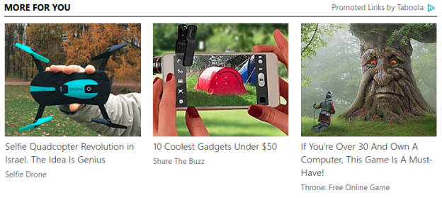
Examples of advertisements placed in Taboola’s “Promoted Links” box. Notice that each advertisement contains both a title and an appealing image.
Given an advertisement title (for example “15 healthy dishes you must try”), the advertiser has endless possibilities of choosing the image thumbnail to accompany it, clearly some more clickable than others. One can apply best practices in choosing the thumbnail, but manually searching for the best image (out of possibly thousands that fit a given title) is time consuming and impractical. Moreover, there is no clear way of quantifying how much a given image is related to a title and more importantly – how clickable the image is, compared to other options.
To Alleviate this problem, we developed a text to image search algorithm that given a proposed title, scans an image gallery to find the most suitable images and estimates their expected click through rate (a common marketing metric depicting the amount of user clicks per a fixed number of advertisement displays).
For example, here are the images returned by our algorithm for the query title “15 healthy dishes you must try” along with their predicted Click Through Ratio (CTR):
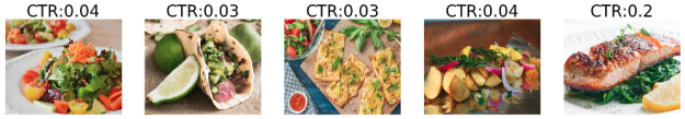
Examples of images returned by our algorithm for the title query “15 healthy dishes you must try” along with their predicted Click Through Ratio (CTR). Notice that the images nicely fit the semantics of title.
Method
In a nutshell, our pipeline is composed of extracting title embeddings, extracting image embeddings and learning two transformations to map those embeddings to a joint space. This is done in training time. In test time, we compute the query title embedding and return the most similar images in the joint image-title space. We elaborate on each of these steps below.
Embeddings
First, let us consider the concept of embeddings. An embedding function is a function that receives an item (be it image or text) and produces a numerical vector for the item that captures its semantic meaning, such that if two items are semantically similar – then their vectors would be close. For example the two embedding vectors for the two titles “Kylie Jenner, 19, Buys Fourth California Mansion at $12M” and “18 Facts about Oprah and her Extravagant Lifestyle” should be similar, or close in the embedding space, while the vectors for the titles “New Countries that are surprisingly good at these sports” and “Forgetting things? You should read this!” should be very different, or far away from each other in the embedding space. Similarly, the vectors for following two images
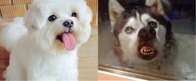
Example of two images which are semantically similar, but extremely different in terms of the raw pixel information
should be close in the embedding space since their semantic meaning is the same (dogs making funny faces), even though the specific image pixel values are vastly different.
At first glance, one might consider such an embedding function to be very explicit: for example, counting the number of faces in an image, the number of nouns in a sentence, perhaps creating a list of the objects in an image. Such explicit functions are in fact extremely hard to implement and in practice do not preserve semantics very well, at least not in a way which easily allows us to compare them. In practice embedding functions represent the information of the item in a much more implicit manner, as we will see next.
More concretely, let 


Image embedding
Pre-trained Convolutional Neural Networks have shown to be extremely useful in obtaining strong image representation [4]. In our framework, we use a ResNet 152 [5] model pretrained on the Imagenet Large Scale Visual Recognition Challenge (ILSVRC) dataset[6]. Each image is fed to the pretrained network and we take the activation of the res5c layer as a 2048 embedding vector. To better illustrate the quality of the embeddings, we implement a simple image search demo on our own Taboola image dataset – given a query image we compute it’s embedding vector and return the images with the closest embedding vectors. Here are the 4 most similar images to several image queries (the query is the leftmost image):
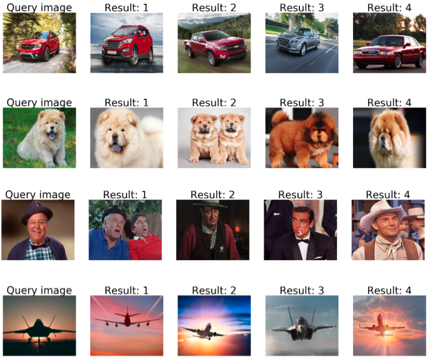
Given a query image, we compute it’s embedding vector and return the images with the closest embedding vector in the embedding space. In each row, the leftmost image is the query image, the four other images are the most similar images to the query according to their embedding vectors.
Title embedding
A number of sentence embedding methods were proposed in the literature[8-10]. However, we found Infersent [11] to be particularly useful in our application. While common approaches to sentence representation are unsupervised or leverage the structure of the text for supervision (i.e: self-supervised methods), Infersent[11] trains sentence embeddings in a fully supervised manner. To this end, [11] leverages the SNLI [12] dataset which composes of 570K pairs of sentences with a label depicting the relationship between them (contradiction, neutral or entailment). The authors train a number of different models on the SNLI dataset and test their performance as sentence embeddings on a variety of downstream NLP tasks. The best performance was obtained by training a BiLSTM and taking a max-pooling of it’s hidden states as a representation.
To illustrate the quality of the embeddings, below are examples of title queries and their nearest neighbors using Infersent[11] as a sentence embedding:
Query: “15 Adorable Puppy Fails The Internet Is Obsessed With”
- NN1: 18 Puppy Fails That The Internet Is Obsessed With
- NN2: 13 Adorable Puppy Fails That Will To Make You Smile
- NN3: 16 Dog Photoshoots The Internet Is Absolutely Obsessed With
Query: “10 Negative Side Effects of Low Vitamin D Levels”
- NN1: How to Steer Clear of Side Effects From Blood Thinners
- NN2: 7 Signs and Symptoms of Vitamin D Deficiency People Often Ignore
- NN3: 8 Facts About Vitamin D and Rheumatoid Arthritis
Matching titles and images
Given a query title, we would like to fit it with the most relevant images. For example, the query “20 new cars to buy in 2018” should return images of new and shiny high end cars. As mentioned before, our analysis of titles and images is not explicit, meaning that we do not explicitly detect the objects and named entities of the titles and match it with images containing the same objects. Instead, we rely on the title and image embeddings which implicitly capture their semantics.
Next, we need to have a better grasp of what does it mean that a title corresponds to an image. To this end, we built a large training set composed of pairs of title and image from advertisements that appeared in the Taboola widget. Denote by 


Given this definition, as a naive first solution we can apply the following pipeline: given a title 


While this is a sound solution, it does not fully leverage our training set since for each query it uses information from only one <title, image> training pair. Indeed, our experiments showed that the images suggested in this manner were far less suitable than images that were suggested from an approach which uses the entire training gallery. In order to leverage the entire training set of titles and images, we would like to implicitly capture the semantic similarity of titles, images and the given correspondence between them in our training set. To this end, we employ an approach that learns a joint title-image space in which both the titles and the images reside. This allows us to directly measure distance between titles and images and in particular, given a query title, find its nearest neighbor image. We will later describe the manner in which this space is learned.
To better illustrate the difference between the two approaches, consider for example the query “30 Richest Actresses in America”. We would like to return the images from our gallery that are most similar to the query. In the first approach we would find the most similar title from the gallery via their embedding distance. After computing embedding distance we found that the most similar title is “The 30 Richest Canadians Ranked By Wealth”. That title appeared in several advertisements, along with the images shown below:

Images returned by the naive algorithm for the query “30 Richest Actresses in America”. Notice that the images are not related to the query at all. Later we will show that the proposed approach achieves far better results.
Obviously, those images have nothing to do with the query title “30 Richest Actresses in America”. This is not very surprising, since while the nearest neighbor title “The 30 Richest Canadians Ranked By Wealth” is the most similar title in our gallery, it is not similar enough to the query. However, there might be other images in the gallery that are more semantically similar to the query title “30 Richest Actresses in America”. Notice that we are considering here both similarities between a pair of titles and similarities a title and an image, since as we will see next, the learned joint space allows us to consider both types of similarities.
As reference, here are the results returned by our method (which is explained next) for the title “30 Richest Actresses in America”.

Images returned by searching in the proposed joint title-image space algorithm for the query “30 Richest Actresses in America”. Notice the returned images are far more suitable than the ones returned by the naive algorithm.
Learning a joint space
Assume we have 


Numerous methods for obtaining such mappings exist [13-16, see 19 for an extensive survey]. However, we found a simple statistical method to be useful in our application. To this end, we employ Canonical Correlation Analysis (CCA) [17].
Let ![T=\left[t_1,t_2,\dots,t_n \right]](https://s0.wp.com/latex.php?latex=T%3D%5Cleft%5Bt_1%2Ct_2%2C%5Cdots%2Ct_n+%5Cright%5D+&bg=ffffff&fg=444444&s=0&c=20201002)
![M= \left[m_1,m_2,\dots,m_n \right]](https://s0.wp.com/latex.php?latex=M%3D+%5Cleft%5Bm_1%2Cm_2%2C%5Cdots%2Cm_n+%5Cright%5D&bg=ffffff&fg=444444&s=0&c=20201002)


Click Through Rate estimation
Now, given a proposed image, we would like to estimate it’s Click Through Rate (CTR) – the amount of clicks divided by the number of appearances. Many of the images in our gallery already appeared in campaigns, so we can use their historic data. For others, we train a simple linear Support Vector Machine regression model [18] based on their image embeddings.
Full image search pipeline
Our final image search pipeline works as follows: First, we take a large gallery of titles and images, run the ResNet 152[5] model and the InferSent[11] model to obtain image and title embeddings. Next, we apply CCA[17] to learn two linear projections –
Now, given a new title text by the advertiser, we run the InferSent[11] model to obtain its embedding 


Examples:
Now for the fun part. Here are some quantitative results of our pipeline using real titles that appeared in some of our recommendations. For each title, we present the top 8 images returned by our system with their predicted click through ratio.
Query title: “30 Richest Actresses in America”, images returned:

Images returned by our system for the query “30 Richest Actresses in America” along with their predicted CTR. Notice this is the same title we discussed earlier when comparing our approach with the naive solution. Here we also show the predicted CTR. We assume our model mistook Steven Tyler’s for a female actress due to his long hair…
Query title: “Baby Born With White Hair Stumps Doctors”, images returned:

Images returned by our system for the query “Baby Born With White Hair Stumps Doctors” along with their predicted CTR. Note that some of the rightmost images are a bit off since they are farther away from the title embedding in the joint space.
Our algorithm also works for longer titles, for example the query title: “Now You Can Turn Your Passion For Helping Others Into A Career – Become A Nurse 100% Online. Find Enrollment & Scholarships Compare Schedules Now!”, images returned:

Images return by our system for the query “Now You Can Turn Your Passion For Helping Others Into A Career – Become A Nurse 100% Online. Find Enrollment & Scholarships Compare Schedules Now!” along with their predicted CTR.
Query title: “20 Ridiculously Adorable Pet Photos That Went Viral”, images returned:
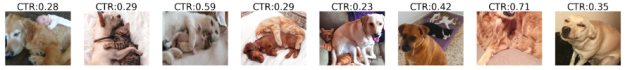
Images return by our system for the query “20 Ridiculously Adorable Pet Photos That Went Viral” along with their predicted CTR.
Query title: “Don’t Miss this Incredible Offer if You Fly with Delta Ends 11/8!”, images returned:

Images returned by our system for the query “Don’t Miss this Incredible Offer if You Fly with Delta Ends 11/8!” along with their predicted CTR.
Summary
Our goal in this post was to illustrate our system for solving a real world difficulty of image search through free text, specifically to be used by advertisers to optimize which images to use for a given advertisement.
While we have developed the system for solving our needs, it is not tailored in any way to advertising and can be used for implementing image search in other domains and industries.
In its current implementation, our system returns the K most similar images for a given query without any other considerations. In future work we intend to add a functionality of controlling how versatile the returned images will be relative to their semantic similarity with the title (i.e. : return a set of images which might fit the title less well, but are versatile and provide the advertiser with more options).
Acknowledgments
The work described above has been done as part of my internship at Taboola. A less technical version of this blog post is also available at Taboola tech blog. I would like to thank Dan Friedman and Yoel Zeldes for their comments and discussion regarding this and other projects I’ve been involved in at Taboola.
References
[1] Dalal, Navneet, and Bill Triggs. “Histograms of oriented gradients for human detection.” Computer Vision and Pattern Recognition, 2005. CVPR 2005. IEEE Computer Society Conference on. Vol. 1. IEEE, 2005.
[2] Ojala, Timo, Matti Pietikäinen, and David Harwood. “A comparative study of texture measures with classification based on featured distributions.” Pattern recognition 29.1 (1996): 51-59.
[3] Csurka, Gabriella, et al. “Visual categorization with bags of keypoints.” Workshop on statistical learning in computer vision, ECCV. Vol. 1. No. 1-22. 2004.
[4] Razavian, Ali Sharif, et al. “CNN features off-the-shelf: an astounding baseline for recognition.” Computer Vision and Pattern Recognition Workshops (CVPRW), 2014 IEEE Conference on. IEEE, 2014.
[5] He, Kaiming, et al. “Deep residual learning for image recognition.” Proceedings of the IEEE conference on computer vision and pattern recognition. 2016.
[6] Russakovsky, Olga, et al. “Imagenet large scale visual recognition challenge.” International Journal of Computer Vision 115.3 (2015): 211-252.
[7] Maaten, Laurens van der, and Geoffrey Hinton. “Visualizing data using t-SNE.” Journal of machine learning research 9.Nov (2008): 2579-2605.
[8] Le, Quoc, and Tomas Mikolov. “Distributed representations of sentences and documents.” International Conference on Machine Learning. 2014.
[9] Kiros, Ryan, et al. “Skip-thought vectors.” Advances in neural information processing systems. 2015.
[10] Hill, Felix, Kyunghyun Cho, and Anna Korhonen. “Learning Distributed Representations of Sentences from Unlabelled Data.” Proceedings of NAACL-HLT. 2016.
[11] Conneau, Alexis, et al. “Supervised Learning of Universal Sentence Representations from Natural Language Inference Data.” Proceedings of the 2017 Conference on Empirical Methods in Natural Language Processing. 2017.
[12] Bowman, Samuel R., et al. “A large annotated corpus for learning natural language inference.” arXiv preprint arXiv:1508.05326 (2015).
[13] Chandar, Sarath, et al. “Correlational neural networks.” Neural computation 28.2 (2016): 257-285.
[14] Wang, Weiran, et al. “On deep multi-view representation learning.” International Conference on Machine Learning. 2015.
[15] Yan, Fei, and Krystian Mikolajczyk. “Deep correlation for matching images and text.” Computer Vision and Pattern Recognition (CVPR), 2015 IEEE Conference on. IEEE, 2015.
[16] Eisenschtat, Aviv, and Lior Wolf. “Linking Image and Text With 2-Way Nets.” Proceedings of the IEEE Conference on Computer Vision and Pattern Recognition. 2017.
[17] Vinod, Hrishikesh D. “Canonical ridge and econometrics of joint production.” Journal of econometrics 4.2 (1976): 147-166.
[18] Cortes, Corinna, and Vladimir Vapnik. “Support-vector networks.” Machine learning 20.3 (1995): 273-297.
[19] Li, Yingming, Ming Yang, and Zhongfei Zhang. “Multi-view representation learning: A survey from shallow methods to deep methods.” arXiv preprint arXiv:1610.01206 (2016).
[20 ] Lai, Pei Ling, and Colin Fyfe. “Kernel and nonlinear canonical correlation analysis.” International Journal of Neural Systems 10.05 (2000): 365-377.
[21] Andrew, Galen, et al. “Deep canonical correlation analysis.” International Conference on Machine Learning. 2013.
