In the last post we talked about age and gender classification from face images using deep convolutional neural networks. In this post we will show a similar approach for emotion recognition from face images that also makes use of a novel image representation based on mapping Local Binary Patterns to a 3D space suitable for finetuning Deep Convolutional Neural Networks [8]:

Local Binary Patterns (LBP) Mapping
Our method was presented in the following paper:
Gil Levi and Tal Hassner, Emotion Recognition in the Wild via Convolutional Neural Networks and Mapped Binary Patterns, Proc. ACM International Conference on Multimodal Interaction (ICMI), Seattle, Nov. 2015
For code, models and examples, please see our project page.
Acknowledgements
The presented work was developed and co-authored with Prof. Tal Hassner.
I would also like to thank David Beniaguiev for his useful advice regarding this and other research projects.
Introduction
Automatic facial expression had been subject to much research in recent years. However, performance of current algorithms is still far worse than human performance and much progress still need to be made in order to meet human level. This is especially noteworthy since recent works in the related task of face-recognition reported super-human performance [1,2,3].
Motivated by the success of deep learning method in various classification problems (e.g object classification [4] , human pose estimation [5], face parsing [6], facial keypoint detection [7], action classification [8], age and gender classification [9] and many more) we propose to use Deep Convolutional Neural Networks [10] for facial emotion recognition. Moreover, we present a novel mapping from image intensities to an illumination invariant 3D space based on the notion of Local Binary Patterns [11,12,13]. Unlike regular LBP codes, our mapping produces values in a metric space which can be used to finetune existing RGB convolutional neural networks (see the figure above).
We apply our LBP mapping with various LBP parameters to the CASIA WebFace collection [14] and use the mapped images (along with the original RGB images) to train an ensemble of CNN models with different architecture. This allows our models to learn general face representations. We then use the pretrained models to finetune on a much smaller set of emotion labels face images. We demonstrate our method on the Emotion Recognition in the Wild Challenge (EmotiW 15), Static Facial Expression Recognition sub-challenge (SFEW) [15]. Our method achieves an accuracy of 54.5%, which is a 15.3% improvement over the baseline provided by the challenge authors (40% gain in performance).
Method
First, we will give an overview of our method. We assume the input images are converted to grayscale and cropped to the region of the face. Further, the images were aligned using the Zhu and Ramanan facial feature detector [16].
- We begin by extracting LBP [11,12,13] codes as 8 bit binary vector from each pixel.
- Next, LBP codes are transformed to a 3D space by apply Multi-Dimensional Scaling (MDS) using Earth Mover’s Distance as a distance metric.
- The mapped images, along with the original RGB images, are used to train an ensemble of Deep Convolutional Neural networks. The final predictions is then a weighted sum of the predictions of each of the separate networks.
Each of those steps is defined in detail below.
Local Binary Patterns
Local Binary Patterns [11,12,13] capture local texture by considering local image similarity. To produce an LBP code at a certain pixel location, the intensity values of the 8 adjacent pixels are thresholded by the the center pixel intensity. This produces an 8 bit binary vector where each bit is 1 if the corresponding adjacent pixel’s intensity was larger than the center pixel’s intensity and 0 otherwise. This process is depicted in the following illustration:
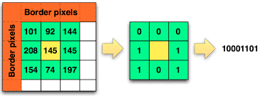
LBP thresholds a small region by the center pixel’s intensity to get a binary value for each pixel.
In the common LBP pipeline, LBP codes are extracted in each pixel location and transformed to decimal values. The image is then divided into regions and for each region a histogram of LBP codes is created. Finally, the different histograms are concatenated to produce a single global descriptor for the image. Here instead we will simply calculate an 8 bit binary vector for each image which we will afterward map into a 3 dimensional space.
Multidimensional Scaling and the Earth Mover’s Distance
After extracting LBP codes in each pixel location, we would like to map the 8 channel binary image to a regular 3 channel image. That would allow us to later use pre-trained network and finetune them to the specific problem at hand. One method for dimensionality reduction is Multi-Dimensional Scaling (MDS) [17,18]. Given a high-dimensional set of data and a similarity matrix describing the similarity distance between each pair of high-dimensional data points, MDS produces a mapping which can transform the high-dimensional dataset to the desired low dimensional space while trying to preserve the distances between each pair of data points. Now, the question that arises is how to choose a suitable similarity metric between the 8 bit LBP codes in a way that appropriately captures their visual similarity?
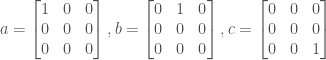
The most straightforward approach would be use the standard euclidean norm, as done in regular images. That would mean to take the decimal value of each LBP code and simply take the absolute values of their difference. However, that would introduce large differences between codes that are actually very similar. We will demonstrate this using a toy example: consider the following three binary LBP codes: a = (1,0,0,0,0,0,0,0,0), b=(0,0,0,0,0,0,0,0), c=(0,0,0,0,0,0,0,1). Clearly, the visual difference between ‘a’ and ‘b’ is the same as the visual difference between ‘b’ and ‘c’ – they only differ in one bit in both cases. Now, let’s compute their euclidean distance: |a-b| = |128-0| = 128, |b-c| = |0 -1| = 1. We get a large difference in euclidean distance for pairs of LBP codes with the actually the same ‘visual’ difference.
A different approach would be to take the difference between the binary 8-bit LBP code which is usually calculated as their Hamming distance – the number of different bits between the two binary vectors which can be computed as the sum of the result of the XOR operation of the two vectors. This metric, however, ignores completely the locations of the bits which are different between the two vectors. This seemingly negligible detail can actually introduce large differences between LBP vectors produced from very similar intensity patterns. To demonstrate this, consider the following three binary 8-bit LBP vectors: a = (1,0,0,0,0,0,0,0,0), b=(0,1,0,0,0,0,0,0), c=(0,0,0,0,0,0,0,1):
The hamming distance between pattern a and patten b is equal to the hamming distance between the pattern a and the pattern c (both equal 1). However, pattern b is different from pattern a by a slight single pixel rotation around the central pixel whereas pattern c is a mirror of pattern a, thus the local patches that produces patterns a and b are more similar than the local patches that produced patterns a and c. Clearly, the spatial location of the different bits also needs to be taken into consideration.
To this end, we find the Earth Mover’s Distance [19] to be suitable to our scenario. Originally, the Earth Mover’s distance was designed to compare histograms in a way that takes into account the spatial location of the bins. The Earth Mover’s Distance can be illustrated by the amount of work needed to align two piles of dirt (representing the two histograms) against each other – the energy of moving dirt takes in consideration both the differences in the piles height in each location, but also how far the dirt needs to be moved.
Training deep networks
Due to the huge number of model parameters, deep CNN are prone to overfitting when they are not trained with a sufficiently large training set. The EmotiW challenge contains only 891 training samples, making it dramatically smaller than other image classification datasets commonly used for training deep networks (e.g, the Imagenet dataset [20]). To alleviate this problem, we train our models in two steps: First, we finetune pre-trained object classification networks on a large face recognition dataset, namely the CASIA WebFace dataset [21]. This allows the network to learn general features relevant for face classification related problems. Then, we finetune the resulting networks for the problem of emotion recognition using the smaller training set given in the challenge. Furthermore, we apply data-augmentation during training by feeding the network with 5 different crops of each image and their mirrors (over-sampling). This is also done in test time and in practice improves the accuracy of the models.
Experiments
We experimented with 4 different network architectures and 5 different image transformations, giving us a total of 20 deep models which we later ensemble by a weighted average of each model’s predictions. The network’s architecture that we used are VGG_S, VGG_M_2048, VGG_M_4096 [22] and GoogleNet[23]. We used mapped LBP transformations with radii of 1, 5 and 10 pixels as well as the original RGB values. Once the networks were trained, we used the validation set to learn a weighted average of their predictions.
Results
The table below lists our results for all the various combinations of image transformation and network architecture:
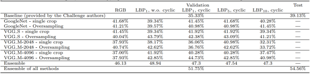
Results of our Emotion Classification method for various network’s architecture and image transformations.
The table seems a bit overloaded with numbers, but one important thing we can notice is that the networks trained on the original RGB images did not give the best results — the best accuracy was obtained by the networks trained on the mapped LBP images.
Below is a histogram of the importance each model got in the final ensemble:
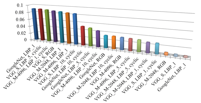
Histogram of the importance of each model in the final ensemble.
Note here that the models trained on the mapped LBP images had the most importance in final ensemble.
Also see below some of the predictions made by our system. In some cases, the faces that the system misclassified are heavily blurred, not correctly cropped or in challenging head pose.

Examples of predictions made by our emotion classification system.
Conclusion
We showed that by applying a certain image transformation, mapped LBP in this case, we can enforce the model to learn different features. This becomes useful when ensembling such models – since each model learned different information, the models complement each other and the accuracy we get when ensembling them is dramatically higher than each model alone. This is evident from our results as our best model achieved an accuracy of 44.73% while our ensemble achieved 51.75% on the validation set. Moreover, we achieved an accuracy of 54.56% which is a 15.36% improvement over the baseline provided by the challenge authors.
References
[1] Schroff, Florian, Dmitry Kalenichenko, and James Philbin. “Facenet: A unified embedding for face recognition and clustering.” arXiv preprint arXiv:1503.03832 (2015).
[2] Sun, Yi, et al. “Deepid3: Face recognition with very deep neural networks.” arXiv preprint arXiv:1502.00873 (2015).
[3] Sun, Yi, Xiaogang Wang, and Xiaoou Tang. “Deeply learned face representations are sparse, selective, and robust.” arXiv preprint arXiv:1412.1265 (2014).
[4] Krizhevsky, Alex, Ilya Sutskever, and Geoffrey E. Hinton. “Imagenet classification with deep convolutional neural networks.” Advances in neural information processing systems. 2012.
[5] Toshev, Alexander, and Christian Szegedy. “Deeppose: Human pose estimation via deep neural networks.” Computer Vision and Pattern Recognition (CVPR), 2014 IEEE Conference on. IEEE, 2014.
[6] Luo, Ping, Xiaogang Wang, and Xiaoou Tang. “Hierarchical face parsing via deep learning.” Computer Vision and Pattern Recognition (CVPR), 2012 IEEE Conference on. IEEE, 2012.
[7] Sun, Yi, Xiaogang Wang, and Xiaoou Tang. “Deep convolutional network cascade for facial point detection.” Computer Vision and Pattern Recognition (CVPR), 2013 IEEE Conference on. IEEE, 2013.
[8] Sun, Yi, Xiaogang Wang, and Xiaoou Tang. “Deep convolutional network cascade for facial point detection.” Computer Vision and Pattern Recognition (CVPR), 2013 IEEE Conference on. IEEE, 2013.
[9] Gil Levi and Tal Hassner, Age and Gender Classification using Convolutional Neural Networks, IEEE Workshop on Analysis and Modeling of Faces and Gestures (AMFG), at the IEEE Conf. on Computer Vision and Pattern Recognition (CVPR), Boston, June 2015.
[10] LeCun, Yann, et al. “Backpropagation applied to handwritten zip code recognition.” Neural computation 1.4 (1989): 541-551.
[11] Ojala, Timo, Matti Pietikäinen, and David Harwood. “A comparative study of texture measures with classification based on featured distributions.” Pattern recognition 29.1 (1996): 51-59.
[12] Ojala, Timo, Matti Pietikäinen, and Topi Mäenpää. “A generalized Local Binary Pattern operator for multiresolution gray scale and rotation invariant texture classification.” ICAPR. Vol. 1. 2001.
[13] Ojala, Timo, Matti Pietikäinen, and Topi Mäenpää. “Multiresolution gray-scale and rotation invariant texture classification with local binary patterns.” Pattern Analysis and Machine Intelligence, IEEE Transactions on 24.7 (2002): 971-987.
[14] Yi, Dong, et al. “Learning face representation from scratch.” arXiv preprint arXiv:1411.7923 (2014).
[15] Dhall, Abhinav, et al. “Video and image based emotion recognition challenges in the wild: Emotiw 2015.” Proceedings of the 2015 ACM on International Conference on Multimodal Interaction. ACM, 2015.
[16] Zhu, Xiangxin, and Deva Ramanan. “Face detection, pose estimation, and landmark localization in the wild.” Computer Vision and Pattern Recognition (CVPR), 2012 IEEE Conference on. IEEE, 2012.
[17] Borg, Ingwer, and Patrick JF Groenen. Modern multidimensional scaling: Theory and applications. Springer Science & Business Media, 2005.
[18] Seber, George AF. Multivariate observations. Vol. 252. John Wiley & Sons, 2009.
[19] Rubner, Yossi, Carlo Tomasi, and Leonidas J. Guibas. “A metric for distributions with applications to image databases.” Computer Vision, 1998. Sixth International Conference on. IEEE, 1998.
[20] Russakovsky, Olga, et al. “Imagenet large scale visual recognition challenge.” International Journal of Computer Vision 115.3 (2015): 211-252.
[21] Yi, Dong, et al. “Learning face representation from scratch.” arXiv preprint arXiv:1411.7923 (2014).
[22] Chatfield, Ken, et al. “Return of the devil in the details: Delving deep into convolutional nets.” arXiv preprint arXiv:1405.3531 (2014).
[23] Szegedy, Christian, et al. “Going deeper with convolutions.” Proceedings of the IEEE Conference on Computer Vision and Pattern Recognition. 2015.

Hi, Thanks for sharing the code. But I got the following error while running lbp_mapping_code.m:
> In pca (line 28)
In mdscale (line 413)
In lbp_mapping_code (line 25)
Operands to the || and && operators must be convertible to logical scalar values.
Error in pca (line 55)
if numvecs<=dim && dim<p
Error in mdscale (line 413)
[~,score] = pca(Y,'Economy',false);
Error in lbp_mapping_code (line 25)
Y=mdscale(cyclic_dist_matrix,3);
Could you help me fix it? Thanks a lot.
Best,
Cindy
Hi, it turns out I have another pca file which has different definition of inputs. Your code works perfectly fine! Thanks a lot.
Glad to hear that, let me know if you have any other issues with the code. Cheers, Gil.
This is probably the best, most concise step-by-step guide I’ve ever seen on how to build a successful blog.
Thanks for sharing!
Thank you for your kind words.
Dear Gil,
Greeting,
I hope you are well.
Can I ask you what is the problem of Descriptor Evaluation code provided by vgg with binary descriptors?
You know, the code does not give good results in the case of a binary descriptor, alike freak, brief, or even latch!
vgg code: http://www.robots.ox.ac.uk/~vgg/research/affine/desc_evaluation.html#code
Do you have any experience regarding this matter?
Many thanks for considering this request,
Best regards,
Mori
Hi,
The code works for binary descriptors as well, but the descriptors should be written as binary strings instead of the uint8 representation (and perhaps change some of the C++ code to replace L2 with hamming distance).
How did you run it? what were the inputs?
Best,
Gil