In the last few posts we introduced the concept of local image descriptors and specifically binary image descriptors. We surveyed notable example of binary descriptors, namely BRIEF[1], ORB[2], BRISK [3] and FREAK[4]. Here, we will both introduce a novel binary descriptor that we have developed and give a full evaluation of several binary and floating point descriptors. We will show that our proposed descriptor – the LATCH descriptor[5] – outperforms the alternatives with similar running times. We will also demonstrate its performance in the real world application of 3D reconstruction from multiple images.
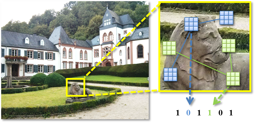
Given an image patch centered around a keypoint, LATCH compares the intensity of three pixel patches in order to produce a single bit in the final binary string representing the patch. Example triplets are drawn over the patch in green and blue
Our proposed LATCH descriptor was presented in the following paper:
Gil Levi and Tal Hassner, LATCH: Learned Arrangements of Three Patch Codes, IEEE Winter Conference on Applications of Computer Vision (WACV), Lake Placid, NY, USA, March, 2016
Here is a short video of me presenting LATCH at the WACV 16 conference (I apologize for the technical problems in the video).
Our LATCH descriptor has already been officially integrated into OpenCV3.0 and has even won the CVPR 2015, OpenCV State of the Art Vision Challenge, in the Image Registration category !
Also, see CUDA (GPU) implementation of the LATCH descriptor and a cool visual odometry demo, both by Christopher Parker.
For more information, please see LATCH project page.
Acknowledgements
The LATCH descriptor was developed along with my master thesis supervisor, Prof. Tal Hassner. I would like to take this opportunity and thank him again for his support, insight and endless patience.
I would also like to thank David Beniaguiev for his useful advice regarding this and other research projects.
Survey of Related Image Descriptors
Histogram based descriptors (SIFT and friends)
One of the key problems in Computer Vision, that is a common underline to the vast majority of Computer Vision application (for example, 3D reconstruction, Face Recognition, Dense Correspondence, etc.), is that of representing local image patches. Numerous attempts have been made at obtaining a discriminative local patch representation, which is both invariant to various image transformations as well as efficient to extract and match.
Until recently [1], the common approach for representing local patches was through the use of Histograms of Oriented Gradients. One of the early works in this approach is the Scale Invariant Feature Transform (SIFT) [11] which computes an 8 bins histogram of gradients orientation in each cell of 4×4 grid. Once histograms are computed, they are normalized and concatenated into a single 128-dimensional descriptor that is commonly compared using the L2 metric.
Since the use of gradients is time-consuming, the Speeded Up Robust Feature (SURF) [12] descriptor make use of integral images in order to speed up feature extraction. It is important to note that although SURF speeds up descriptors extraction, the matching phase which is an order of O(n^2) in the number of image descriptors, still uses the expensive and time consuming L2 metric.
Other notable examples in this line of work include the Gradient Location and Orientation Histogram (GLOH) [13] descriptor which replaces SIFT’s 4×4 rectangular grid by a log-polar grid to improve rotation invariance as well as PCA-SIFT [14] which builds upon SIFT, but uses the PCA dimensionality reduction technique to improve its distinctiveness and to reduce it’s size.
Binary Descriptors
Though much work have been devoted in obtaining strong representations [11, 12, 13, 14], it is was only until recently that a major improvement in both running times and memory footprint has been obtained with the emergence of the binary descriptors [1 ,2, 3, 4]. Instead of expensive gradients operations, Binary Descriptors make use of simple pixel comparison which result in binary strings of typically short length (commonly 256 bits). The resulting binary representation hold some very useful properties:
- Pixel comparisons are much faster than gradients operations, thus binary descriptors can be extracted in a fraction of the time required to compute the common gradient based descriptors.
- Matching binary representations is done using hamming distance which is much faster to compute than the L2 metric. The matching speed-up is ever more dramatic considering that Hamming distance can be computed using a single POPCNT instruction on most processors.
- Whereas a single gradient based descriptor commonly require 64 or 128 floating point values to store, a single binary descriptors requires only 512 bits – 4 to 8 times less.
Those characteristics are of particular importance for real-world real-time applications that commonly require fast processing of an increasing amount of data, often on mobile devices with limited storage and computational power.
One of the early works in this line of work was the Binary Robust Independent Elementary Features (BRIEF) descriptor [1]. BRIEF operates by comparing the same set of smoothed pixel pairs for each local patch that it describes. For each pair, if the first smoothed pixel intensity is larger than that of the second, BRIEF writes 1 in the final descriptor string and 0 otherwise. The sampling pairs are chosen randomly, initialized only once and used for each image and local patch.
The Oriented fast and Rotated BRIEF (ORB) descriptor [2] builds upon BRIEF by adding a rotation invariance mechanism that is based on measuring the patch orientation using first order moments. ORB also uses unsupervised learning to learn the sampling pairs.
Instead of using arbitrary sampling pairs the Binary Robust Invariant Scalable Keypoints (BRISK) descriptor [3] uses a hand-crafted sampling pattern that is composed of set of concentric rings. BRISK uses the long-distance sampling pairs to estimate the patch orientation and the short distance sampling pairs to construct the descriptor itself through pixel intensity comparisons.
The Fast REtina Keypoint (FREAK) descriptor [4] is similar to BRISK by having a hand crafted sampling pattern. However, it’s sampling pattern is motivated by the retina structure, having exponentially more sampling points toward the center, and similar to ORB, FREAK also uses unsupervised learning to learn a set of sampling pairs.
Similar to BRIEF, the Local Difference Binary (LDB) descriptor was proposed in [15] where instead of comparing smoothed intensities, mean intensities in grids of 2 × 2, 3 × 3 or 4 × 4 pixels were compared. Also, in addition to the mean intensity values, LDB also compares the mean values of horizontal and vertical derivatives, amounting to 3 bits per comparison.
Building upon LDB, the Accelerated KAZE (A-KAZE) descriptor[10] uses the A-KAZE detector estimation of orientation for rotating the LDB grid to achieve rotation invariance. In addition, A-KAZE also uses the A-KAZE detector’s estimation of patch scale to sub-sample the grid in steps that are a function of the patch scale.
On a different line of work are recent approaches for extracting binary descriptors, which instead of using pixel comparison, use linear/non-linear projections followed by threshold operations to achieve binary representations. One of the first methods in this line of work is the LDA-Hash [15] descriptor which first extract SIFT descriptors in the image, then projects the descriptors to a more discriminant space and finally thresholds the projected descriptors to obtain a binary representation.
Instead the intermediate step of extracting floating point descriptors, the DBRIEF [7] descriptor projects the patches directly, where the projections are computed as a linear combination of a small number of simple filters.
Finally, the BinBoost [8,9] descriptor projects the image patch to a binary vector by applying a set of hash functions learned through boosting. The hash functions are a signed operation on a linear combination of a set of gradient-based filters.
Though some works in that line claim improved performance, their drawback is an increase in descriptor extraction time, which might render them unsuitable for real-time applications.
We propose a novel binary descriptors that belongs to the earlier family of binary descriptors, i.e. binary descriptors that use fast pixel comparisons. However, we propose to use small patch comparisons, rather than pixel comparisons, and use triplets rather than pairs of sampling points. We also present a novel method for learning an optimal set of sampling triplets. The proposed descriptor is appropriately dubbed LATCH – Learned Arrangements of Three patCHes codes.
Again, the full details of our approach including evaluation and comparison with other binary descriptors can be found in the following paper:
Levi, Gil, and Tal Hassner. “LATCH: Learned Arrangements of Three Patch Codes.” arXiv preprint arXiv:1501.03719 (2015). (link to project page)
Method
First, we give a reminder of binary descriptors design (the reader may also refer to my earlier post on introduction to binary descriptors). The goal of binary descriptors is to represent local patches by a binary vectors that can be quickly matched using Hamming distance (the sum of the XOR operation). To this end, a binary descriptors uses a set of sampling pairs S = (s1 , s1 , . . . , sn), where each si is a pair of two pixel locations defining where to sample in a local patch. For each sampling pair, the descriptor compares the intensity in the location of the first pixel to that of second pixel – if the intensity is greater then it assigns 1 in the final descriptor and 0 otherwise. The comparisons result in a binary string which can be compared very efficiently using Hamming distance.
Even though some variants of binary descriptors smooth the mini-patch around each sampling point, we note that comparing single pixels might cause the representation to be sensitive to noise and slight image distortions. We propose instead to compare the mini-patches themselves and in order to increase the spatial support of the binary tests, we use triplets of mini-patches, rather than pairs. Moreover, we devise a novel method for learning an optimal set of triplets using supervised learning. This is in contrast to the learning methods of ORB [1] and FREAK [4] which are not supervised.
From pairs to triplets
As described above, the LATCH descriptor uses triplets of mini-patches. To create a descriptor for 512 bits, LATCH uses 512 triplets, where each triplet defines the location of three mini-patches of size K x K, we assume 7×7. In each triplet, one of the mini-patches is denoted an ‘anchor’ and the other two mini-patches are denoted as ‘companions’. We will denote the anchor as ‘a’ and the companions as ‘c1’ and ‘c2’.
For each of the 512 triplets, we test if the companion patch ‘c1’ is more similar to the anchor ‘a’ than the second companion ‘c2’. For measuring similarity between patches, we use the sum-of-squared differences (denoted SSD).
To summarize, the LATCH descriptor uses a predefined set of 512 triplets, defining where to sample in a local image patch. Given a local patch, the LATCH descriptor goes over all 512 triplets. For each triplet, if the SSD between the anchor ‘a’ and the companion ‘c1’ is smaller than the SSD between ‘a’ and the second companion ‘c2’, then we write ‘1’ in the resulting bit. If not, we write ‘0’. The distance between LATCH descriptors is computed as their hamming distance, as with the other binary descriptors.
Learning patch triplet arrangements
Assume we would like to represent a local patch of size 48 x 48. Considering all the possible pixel triplets in that region will amount to an enormous number of triplet possibilities. Since binary descriptors typically require no more than 256 bits, a method for selecting an optimal set of triplets is required.
To this end, we leverage the labeled data of the the same/not-same patch dataset of [16]. The dataset consists of corresponding patches sampled from 3D reconstructions of three popular tourist sites. For each of the three sets, predefined sets of 250K pairs of same and not-same patches were gathered. A ‘same’ patch pair are simply two patches that are visually different (by zoom, illumination or viewpoint), but both correspond to the same real-world 3D point in space. A ‘Not-Same’ patch pair are two patches that correspond to entirely different 3D locations.
Below are examples of same and not-same pair patches – the left figure presents examples of ‘same’ patch pairs and the right figure presents examples of ‘not-same’ patch pairs. Note that the images in each ‘same’ patch pair indeed belong to the same ‘real-world’ patch, but are different in illumination, blur, view-point, etc.

Examples of same and not-same pair patches – the left figure presents examples of ‘same’ patch pairs and the right figure presents examples of ‘not-same’ patch pairs
We randomly draw a set of 56,000 candidate arrangements. Each arrangements defines where to sample the anchor mini-patch and its two companion mini-patches. We then go over all the 56K candidate arrangements and apply each one on the set of 500K pairs of same and not-same patch pairs. The quality score of an arrangement is then defined by the number of times it yielded the same binary bit for the two ‘same’ patch pairs and the number of times it yielded different binary bits for the two ‘not-same’ patch pairs.
We would want to choose the bits with the highest quality score, but that could lead to choosing highly correlated arrangements. Two arrangements can have a very high quality score, but being highly correlated, the second arrangement will contribute very little additional information on the patch given we already computed the first arrangement. To avoid choosing highly correlated arrangements, we follow the method used by ORB [2] and FREAK [4] and add arrangements incrementally, avoiding from adding a new arrangement if it’s correlation with at least one of the previously added arrangements is larger than a predefined threshold.
Experimental results
We have tested our proposed LATCH descriptor on two standard publicly available benchmarks and compared it to the following binary image descriptors: BRIEF [1], ORB [2], BRISK [2], FREAK [4], A-KAZE [10], LDA-HASH/DIF [15], DBRIEF [7] and BinBoost [8,9]. To also compare against floating point descriptors we have included SIFT [11] and SURF [12] in our evaluation.
If not mentioned otherwise, we extracted LATCH from 48×48 patches using a 32-byte (256 bits) representation with mini-patches of 7×7 pixels. For all the descriptors we used the efficient C++ code available from OpenCV or from the various authors with parameters left unchanged.
Running times
We start by a run time analysis of the various descriptors included in our evaluation. We measured the time (in milliseconds) required to extract a single descriptor (averaged on a large set of patches).
The results are listed in the table below. Evidently, there is a large difference in running times between the ‘pure’ comparison-based descriptors and the projection based binary descriptors.
| Descriptor | Running time (ms) |
| SIFT [11] | 3.29 |
| SURF [12] | 2.11 |
| LDA-HASH [15] | 5.03 |
| LDA-DIF [15] | 4.74 |
| DBRIEF [7] | 8.75 |
| BinBoost [8,9] | 3.29 |
| BRIEF [1] | 0.234 |
| ORB [2] | 0.486 |
| BRISK [3] | 0.059 |
| FREAK [4] | 0.072 |
| A-Kaze [10] | 0.069 |
| LATCH [5] | 0.616 |
The Mikolajczyk benchmark
The Mikolajczyk benchmark was introduced in [13] and has since become a standard benchmark for evaluating local image descriptors (I also used it in my post on adding rotation invariance to the BRIEF descriptor)
The Mikolajczyk benchmark is composed of 8 image sets, each containing 6 images that depict an increasing degree of a certain image transformation:
- Bark – zoom + rotation changes.
- Bikes – blur changes.
- Boat – zoom + rotation changes.
- Graffiti – viewpoint changes.
- Leuven – illumination changes.
- Trees – blur changes.
- UBC – JPEG compression
- Wall – viewpoint changes.
The figure below illustrates example images from each set. In the upper row is the first image from each set, in the bottom row is another image from the set. Note the increasing degree of transformation in each set.
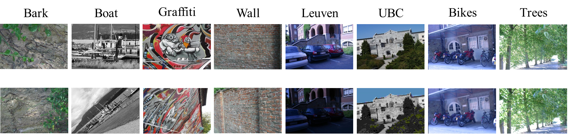
Example images from each set of the Mikolajczyk benchmark
The protocol for the benchmark is the following: in each set, we detect keypoints and extract descriptors from each of the images, then compare the first image to each of the remaining five images and check for correspondences. The benchmark includes known ground truth transformations (homographies) between the images, so we can compute the percent of the correct matches and display the performance of each descriptor using recall vs. 1-precision curves.
Below is a table summarizing the area under the recall vs. 1-precision curve for each of the sets, averaged over the five image pairs – higher values means the descriptor performs better. Recall vs. 1-precision graphs for the sets ‘Bikes’ and ‘Leuven’ are below.
| Descriptor | Bark | Bikes | Boat | Graffiti | Leuven |
| SIFT [11] | 0.077 | 0.322 | 0.080 | 0.127 | 0.130 |
| SURF [12] | 0.071 | 0.413 | 0.088 | 0.133 | 0.300 |
| LDA-HASH [15] | 0.199 | 0.466 | 0.269 | 0.155 | 0.303 |
| LDA-DIF [15] | 0.197 | 0.472 | 0.278 | 0.170 | 0.435 |
| DBRIEF [7] | 0.000 | 0.025 | 0.001 | 0.008 | 0.010 |
| BinBoost [8,9] | 0.055 | 0.344 | 0.083 | 0.132 | 0.338 |
| BRIEF [1] | 0.055 | 0.353 | 0.050 | 0.102 | 0.227 |
| ORB [2] | 0.032 | 0.208 | 0.048 | 0.062 | 0.118 |
| BRISK [3] | 0.015 | 0.138 | 0.026 | 0.071 | 0.161 |
| FREAK [4] | 0.019 | 0.145 | 0.034 | 0.101 | 0.194 |
| A-Kaze [10] | 0.022 | 0.326 | 0.005 | 0.048 | 0.138 |
| LATCH [5] | 0.065 | 0.415 | 0.057 | 0.119 | 0.374 |
| Descriptor | Trees | UBC | Wall | Average |
| SIFT [11] | 0.047 | 0.130 | 0.138 | 0.131 |
| SURF [12] | 0.046 | 0.268 | 0.121 | 0.180 |
| LDA-HASH [15] | 0.110 | 0.393 | 0.268 | 0.270 |
| LDA-DIF [15] | 0.101 | 0.396 | 0.260 | 0.289 |
| DBRIEF [7] | 0.001 | 0.031 | 0.002 | 0.010 |
| BinBoost [8,9] | 0.037 | 0.217 | 0.119 | 0.166 |
| BRIEF [1] | 0.060 | 0.178 | 0.141 | 0.146 |
| ORB [2] | 0.027 | 0.121 | 0.050 | 0.083 |
| BRISK [3] | 0.018 | 0.131 | 0.038 | 0.075 |
| FREAK [4] | 0.026 | 0.147 | 0.041 | 0.089 |
| A-Kaze [10] | 0.027 | 0.144 | 0.048 | 0.095 |
| LATCH [5] | 0.082 | 0.215 | 0.175 | 0.188 |

Recall vs. 1-precision curves for the set “Bikes”
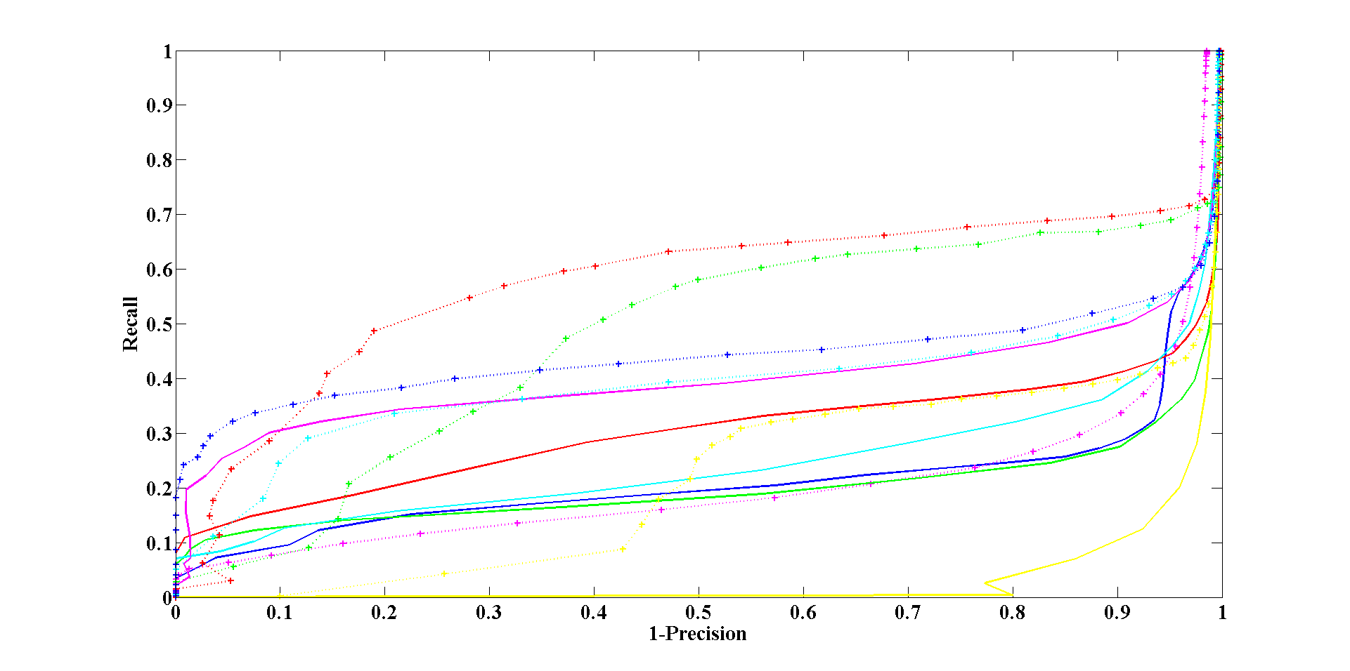
Recall vs. 1-precision curves for the set “Leuven”
Note that LATCH performs much better than most of the alternatives, even better than the floating point descriptors SIFT and SURF. LATCH does perform worse than LDA-HASH/DIF, but their run time is an order of a magnitude slower.
Learning Local Image Descriptors benchmark
Next, we describe our experiments using the data-set from [16], which we also used in learning triplets arrangements. The protocol for this data-set is the following: given a pair of same/not-same patches, extract a single descriptor from each patch and then compute the descriptor distance between the two descriptors. By thresholding over the patch’s distance we can determine if the two patches are considered ‘same’ (distance smaller than the threshold) or ‘not-same’ (distance larger than the threshold). Using the same/not-same labels, we can draw precision vs. recall graphs.
In our experiments, we used the Yosemite set for learning optimal arrangements as well as learning optimal thresholds. Testing was performed on the sets Liberty and Notre-Dame.
The table below presents the results, where we measure accuracy (ACC), area under the ROC curve (AUC) and 95% error-rate (the percent of incorrect matches obtained when 95% of the true matches are found – 95% Err.).
| Notre-Dame | Liberty | |||||
| Descriptor | AUC | ACC | 95% Err. | AUC | ACC | 95% Err. |
| SIFT [11] | 0.934 | 0.817 | 39.7 | .928 | .764 | 40.1 |
| SURF [12] | 0.935 | 0.866 | 41.1 | .911 | .833 | 55.0 |
| LDA-HASH [15] | 0.916 | .830 | 46.7 | .910 | .798 | 48.1 |
| LDA-DIF [15] | 0.934 | .857 | 38.5 | .921 | .836 | 43.1 |
| DBRIEF [7] | 0.900 | .830 | 55.1 | .868 | .794 | 61.5 |
| BinBoost [8,9] | 0.963 | .907 | 21.6 | .949 | .884 | 29.3 |
| BRIEF [1] | 0.889 | .823 | 63.2 | .868 | .798 | 66.7 |
| ORB [2] | 0.894 | .835 | 66.2 | .882 | .822 | 69.2 |
| BRISK [3] | 0.915 | .857 | 57.7 | .897 | .834 | 62.6 |
| FREAK [4] | 0.899 | .835 | 61.5 | .887 | .824 | 65.0 |
| A-Kaze [10] | 0.885 | .806 | 56.7 | .860 | .782 | 63.4 |
| LATCH [5] | 0.919 | .855 | 52.0 | .906 | .838 | 56.7 |
The results above show the clear advantage of LATCH over the other binary alternatives. Although LATCH performance is worse than BinBoost and LDA-HASH/DIF, as noted above, their improved performance does come at the price of slower running times.
3D reconstruction
One of the common uses of local image descriptors is in structure-from-motion (SfM) applications where multiple images of a scene are taken from many viewpoints, local descriptors are then extracted from each image and a 3D model is generated by triangulating corresponding images location. This task requires descriptors to be both discriminative (so that enough correct matches could be made) and fast to match (so that building the model won’t be time consuming). We have chose to apply LATCH to this applications to demonstrate its advantage in both of this aspects. To this end, we have incorporated LATCH into into the OpenMVG library [17] using their incremental structure from motion chain method. We have compared between the 3D models obtained using SIFT and the 3D models obtained using LATCH in terms of running times and visual quality.
Below are reconstruction results obtained using standard photogrammetry images sets:

3D reconstruction results – comparing SIFT and LATCH

3D reconstruction results – comparing SIFT and LATCH
And here are the measured running times for the reconstruction of each model in seconds (descriptors matching time only) :
| Sequence | SIFT | LATCH |
| Sceaux Castle | 381.63 | 39.05 |
| Bouteville Castle | 4766.22 | 488.70 |
| Mirebeau Church | 3166.35 | 325.31 |
| Saint Jacques | 1651.12 | 169.19 |
Notice that although the visual quality of the 3D models obtained with LATCH and SIFT is similar, the matching time of LATCH is an order of a magnitude faster !
Conclusion
By comparing learned triplets of mini-patches rather than pairs of pixels, our LATCH descriptor achieves improved accuracy in similar running times compared to other binary alternatives.
This was demonstrated both quantitatively on two standard image benchmarks and qualitatively through the real-world application of 3D reconstruction from images sets.
For more details, code and paper, please see LATCH project page.
References
[1] Calonder, Michael, et al. “Brief: Binary robust independent elementary features.” Computer Vision–ECCV 2010. Springer Berlin Heidelberg, 2010. 778-792.
[2] Rublee, Ethan, et al. “ORB: an efficient alternative to SIFT or SURF.” Computer Vision (ICCV), 2011 IEEE International Conference on. IEEE, 2011.
[3] Leutenegger, Stefan, Margarita Chli, and Roland Y. Siegwart. “BRISK: Binary robust invariant scalable keypoints.” Computer Vision (ICCV), 2011 IEEE International Conference on. IEEE, 2011.
[4] Alahi, Alexandre, Raphael Ortiz, and Pierre Vandergheynst. “Freak: Fast retina keypoint.” Computer Vision and Pattern Recognition (CVPR), 2012 IEEE Conference on. IEEE, 2012.
[5] Gil Levi and Tal Hassner, LATCH: Learned Arrangements of Three Patch Codes, IEEE Winter Conference on Applications of Computer Vision (WACV), Lake Placid, NY, USA, March, 2016
[6] Strecha, Christoph, et al. “LDAHash: Improved matching with smaller descriptors.” Pattern Analysis and Machine Intelligence, IEEE Transactions on34.1 (2012): 66-78.
[7] Trzcinski, Tomasz, and Vincent Lepetit. “Efficient discriminative projections for compact binary descriptors.” Computer Vision–ECCV 2012. Springer Berlin Heidelberg, 2012. 228-242.
[8] Trzcinski, Tomasz, et al. “Boosting binary keypoint descriptors.” Computer Vision and Pattern Recognition (CVPR), 2013 IEEE Conference on. IEEE, 2013.
[9] Trzcinski, Tomasz, Mario Christoudias, and Vincent Lepetit. “Learning Image Descriptors with Boosting.” (2014).
[10] P. F. Alcantarilla, J. Nuevo, and A. Bartoli. Fast explicit diffusion for accelerated features in nonlinear scale spaces. In British Machine Vision Conf. (BMVC), 2013
[11] Lowe, David G. “Distinctive image features from scale-invariant keypoints.”International journal of computer vision 60.2 (2004): 91-110.
[12] Bay, Herbert, Tinne Tuytelaars, and Luc Van Gool. “Surf: Speeded up robust features.” Computer vision–ECCV 2006. Springer Berlin Heidelberg, 2006. 404-417.
[13] Mikolajczyk, Krystian, and Cordelia Schmid. “A performance evaluation of local descriptors.” Pattern Analysis and Machine Intelligence, IEEE Transactions on27.10 (2005): 1615-1630.
[14] Ke, Yan, and Rahul Sukthankar. “PCA-SIFT: A more distinctive representation for local image descriptors.” Computer Vision and Pattern Recognition, 2004. CVPR 2004. Proceedings of the 2004 IEEE Computer Society Conference on. Vol. 2. IEEE, 2004.
[15] Yang, Xin, and Kwang-Ting Cheng. “LDB: An ultra-fast feature for scalable augmented reality on mobile devices.” Mixed and Augmented Reality (ISMAR), 2012 IEEE International Symposium on. IEEE, 2012.
[16] Brown, Matthew, Gang Hua, and Simon Winder. “Discriminative learning of local image descriptors.” Pattern Analysis and Machine Intelligence, IEEE Transactions on 33.1 (2011): 43-57.
[17] Moulon, Pierre, Pascal Monasse, and Renaud Marlet. “Adaptive structure from motion with a contrario model estimation.” Computer Vision–ACCV 2012. Springer Berlin Heidelberg, 2013. 257-270.

Pingback: Age and Gender Classification using Deep Convolutional Neural Networks | Gil's CV blog
Do I understand correctly that for binary descriptors keypoints are detected as a Harris corners?
Thanks.
Hi,
Thank you for your interest in my post.
I didn’t mention it in the post, but in the paper I explain that each descriptor is used with it’s “own” keypoint detector (as it was presented in it’s original paper).
Best,
Gil
Looking at the PDF (http://www.openu.ac.il/home/hassner/projects/LATCH/LATCH.pdf), it looks like LATCH uses the SIFT detector for keypoints? Is that correct?
Yes, but LATCH can be used with any feature detector.
Is LATCH rotation invariant?
Hi Matthew,
Latch is rotation invariant in the sense that it uses the detector’s estimate of the patch’s orientation in order to rotate the patch to the some predefined global orientation.
Best,
Gil
Do you have any comparison between LATCH and other descriptors while using the same detector. ?
Hi Anil,
I’m afraid I don’t have such comparison.
Best,
Gil
Great work of course, and thank you for sharing both code and documentation.
I would like to know if any optimized implementation for android is available or will be addressed in the near future.
Hello, great work I tried to post earlier but did not work. Sorry for the double post.
I’d like to know if a fast (optimized) implementation of LATCH exists, for ARM processors on android smartphones.
Hi,
Thank you for your interest in our project.
You can find here an insanely fast implementation of LATCH:
https://github.com/komrad36/LATCH
and here an even faster implementation of upright LATCH (LATCH without rotation invariance):
https://github.com/komrad36/ULATCH
Both implementations are for CPU, I believe they are protable for ARM.
The implementation was done by a Kareem Omar whom I had the privilege of co-authoring our CUDA LATCH descriptor, which is (as far as I know) the fastest local image descriptor (requires gpu). You can find a more information about those projects in our project page:
http://www.openu.ac.il/home/hassner/projects/LATCH/
Best,
Gil
Pingback: performance evaluation of binary descriptor introducing the latch descriptor | 不分享空間
hi Gil!
personally i’m working on the evaluration of binary descriptor.Are there any codes to evalurate the LATCH using the Oxford dataset in C++?
Hi Alex,
There is code for running LATCH in C++ (in OpenCV) and also code for evaluating descriptors on the Oxford dataset in Maltab (there is no code in C++ as far as I know) here:
http://www.robots.ox.ac.uk/~vgg/research/affine/desc_evaluation.html#code
Best,
Gil
Do you possibly have a copy of the dataset from [16]? The author’s website seems to be down and there seem to be no mirrors.
I could only find the older version of the dataset here: http://phototour.cs.washington.edu/patches/default.htm
Too bad the authors website is down, I hope they will fix it soon. Have you tried mailing them?
It looks like this is the new location:
http://matthewalunbrown.com/patchdata/patchdata.html
Thanks!
can you send me source code of implementing BRISK Descripto
Hi,
The source code for BRISK is available in OpenCV.
Best,
Gil
hey GIl
i found that the final sampling pointS after learning in your LATCH and CLATCH is diifferent.They use differnt learning method?or do i misunderstand something?
Hi Alex,
Thank you for your interest in LATCH and CLATCH. In both implementation the triplets are the same, only encoded different. We did not learn the sampling points again for CLATCH.
Best,
Gil
Hi Gil,
According to the code you provide, I have a detailed understanding of the LATCH descriptor design process. Now I am very interested in learning patch triplet arrangements. But I do not understand how you learn patch triplet arrangements.
Can you send me the source code about how to learn patch triplet arrangements from patch data? I promise they will be used only for research purposed.
Thank you very much for your kind consideration and I am looking forward to your early reply.
Best,
Gil
Hi Wancheng,
Thank you for your interest in LATCH.
I noticed you’ve also mail me, so I’ll respond there.
Best,
Gil
Thanks for the amazingly educative series of blogs. It made things so much clearer. I had one question though, I could not see the BRIEF implementation anywhere on Github. So while doing these analysis did you use your own BRIEF implementation.
Thank you for your interest in my blog.
I used the implementation of BRIEF from OpenCV.
The previous post on FREAK suggests that it outperforms BRISK and BRIEF in the presence of zoom + rotation. But here we see for the bark test case (zoom + rotation), FREAK has a lower recall vs 1.precision value (0.019) when compared to BRIEF (0.055). What am I missing here?
Are you using rotation invariant BRIEF?
Yes
As you wrote yourself in the following question, here I used the rotation invariant version of BRIEF. This is the cause of the discrepancy between the two results.
Hi Gil,
Really very good work with this new binary descriptor and really interesting.
I was wondering about the experimental results on the Oxoford ACRD dataset, also reported in your WACV paper. As you used the Mikolajczyk’s code, which is mainly for floating point descriptors (e.g. SIFT) and consider the ellipse coefficients for the affine transformations, how did you use it with the binary descriptors to obtain Recall vs 1-Precision curves and AUC results? Did you also varying the matching threshold from 0 to 255 bits?
Thank you in advance for your kind consideration.
Best regards,
Alessio
Hi Alessio,
Thank you for your kind words. The ellipse coefficients were taken from the detector used and the matching threshold was varied from 0 to the maximal distance, which is 256.
Best,
Gil
Hi Gil,
Recently I learned about feature detectors and descriptors, I saw on OpenCV about LATCH descriptors.
However, the paper does not mention how to train triplets patch.
If it possible please send me part of the train method document or sample code.
Best regards,
PH-C
Hi PH-C,
The paper illustrates how to learn the triplets in section “3.2. Learning patch triplet arrangements”.
If you have specific questions, you can mail me at gil.levi100@gmail.com.
Best,
Gil
Pingback: [Из песочницы] Введение в задачу распознавания эмоций - Новини дня
Pingback: [Из песочницы] Введение в задачу распознавания эмоций – CHEPA website